As promised earlier this week, I managed to dedicate some time to the release of a new episode of our citizen science project on Hive, that has been designed to take at most one hour of time (let’s restart gently). As I am also currently dealing with the preparation of my presentation at HiveFest, I take the opportunity to mention that all results obtained by the participants to the project will be included in the presentation, and therefore highlighted widely!
For the moment, the project focuses on the simulation of a signal typical of neutrino mass models at CERN’s Large Hadron Collider (the LHC). I recall that neutrinos are massless beasts in the Standard Model of particle physics, despite that they are experimentally known to be massive today. We must then rely on the presence of new particles to provide an origin to their masses.
These new particles yield specific signals at particle colliders, and our project plans to extend one of my previous studies that targets such a signal when it yields the production at the LHC of a pair of particles called (anti)muons. See also here for a Hive blog on that topic.
Within the context of our citizen science project, we will replace these muons/antimuons by electrons, positrons or even by a mixed pair including one muon and one electron or one antimuon and one positron.
[Credits: Original image from geralt (Pixabay)]
In the previous episode, we took as a reference my older publication, and we tried to reproduce the calculation of the production rate of the di-muon signal at the LHC. In addition, we also provided new results suitable for the third operation run of the LHC that started last July (at an unprecedented collision energy).
I was proud to see that a few Hive community members managed to do that, and were then the first people in the world to calculate total production rates at the LHC run 3 of what is called a double-beta process. Today, we continue focusing on the di-muon signal production rate, but we will this time take care of the uncertainties inherent to the calculation.
Episode 6 - Outline
In the rest of this blog, I first explain how precision can be achieved and why what we have done so far is not precise enough. Next, we will redo the calculations done during episode 5, but this time by also estimating the uncertainties on the predictions. In the upcoming episode 7, we will see how to obtain more precise results.
As usual, I begin this post with a recap of the previous episodes of our adventure, which should allow anyone motivated to join us and catch us up. A couple of hours by episode should be sufficient.
- Ep. 1 - Installation of the MG5aMC software allowing for simulations at particle colliders. We got seven reports from the participants (agreste, eniolw, gentleshaid, mengene, metabs, servelle and travelingmercies), among which that of @metabs consists of an excellent documentation on how to get started with a virtual machine running on Windows.
- Ep. 2 - Simulation of 10,000 LHC collisions leading to the production of a top-antitop pair. We got eight reports from the participants (agreste, eniolw, gentleshaid, isnochys, mengene, metabs, servelle and travelingmercies).
- Ep. 3 - Installation of MadAnalysis5, so that detector effects could be simulated, the output of complex simulations reconstructed, and the results analysed. We got seven contributions from the participants (agreste, eniolw, gentleshaid, isnochys, metabs, servelle and travelingmercies).
- Ep. 4 - Investigations of top-antitop production at CERN’s Large Hadron Collider. We got five contributions from the participants (agreste, eniolw, gentleshaid, servelle and travelingmercies). This episode included assignments whose solutions are available here.
- Ep. 5 - A signal of a neutrino mass models at the LHC. We got four reports from the participants (agreste, eniolw, travelingmercies (part 1) and travelingmercies (part 2)). This episode also included assignments, and their solutions are available here.
I cannot finalise this introduction without acknowledging all current and past participants in the project, as well as supporters from our community: @agmoore, @agreste, @aiovo, @alexanderalexis, @amestyj, @darlingtonoperez, @eniolw, @firstborn.pob, @gentleshaid, @gtg, @isnochys, @ivarbjorn, @linlove, @mengene, @mintrawa, @robotics101, @servelle, @travelingmercies and @yaziris. Please let me know if you want to be added or removed from this list.
Towards precision predictions at the LHC
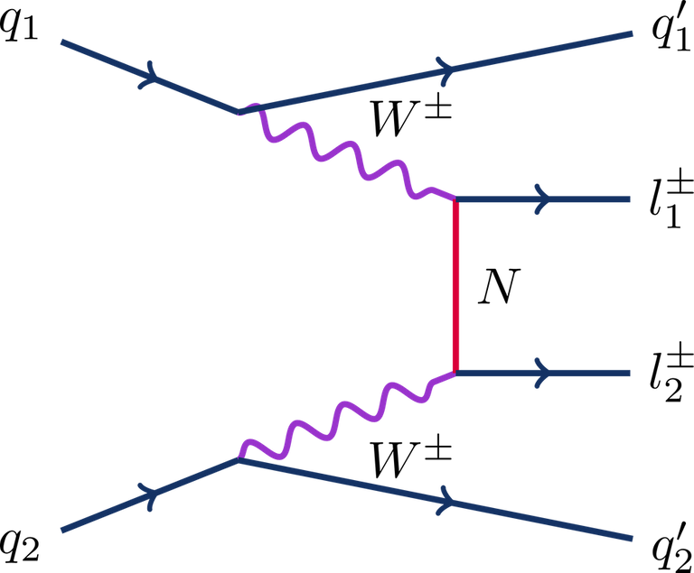
[Credits: CMS-EXO-21-003 (CMS @ CERN)]
The process considered is illustrated by the diagram above. Whereas protons are collided inside the LHC, at high energy they do not scatter as such. It is instead some of their constituents that scatter.
In the specific case of our signal, we must consider collisions between two quarks, one of them being provided by each of the colliding protons. For that reason, the initial state of the process (on the left of the figure) is represented by the symbols q1 and q2.
Then, these initial quarks each emit a very energetic W boson (purple in the figure) by virtue of the weak force, one of the three fundamental forces included in the Standard Model. The two W bosons finally proceed through the core process of interest: they exchange a heavy neutrino N (red in the figure), that is in our model the particle responsible for generating the masses of the neutrinos of the Standard Model.
Such an exchange leads to the production of two leptons of the same electric charge, represented by the symbols l1 and l2 on the right part of the figure. In my older study, we considered that these two leptons were either two muons, or two antimuons.
[Credits: CERN]
I have never mentioned it so far, but the calculation of the production rate associated with the above signal is a perturbative calculation. This means that the result can be written as an infinite series. The first term is the dominant one, and then come subleading corrections, subsubleading corrections, and so on.
Of course, we cannot calculate an infinite series term by term, and we need to truncate it at some point. This naturally leads to uncertainties due to missing higher-order terms. Obviously, the more terms we include, the smaller are the uncertainties (in a series, terms are expected to be smaller and smaller).
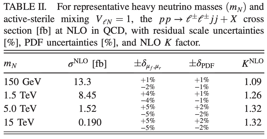
So far, we simply ignored all terms but the leading one, that is represented by the diagram that I have described above. This is called a leading-order calculation. After adding the second term of the series, we perform a next-to-leading-order calculation. It is not that easy to handle numerically, because we have to deal with infinities that cancel each other, which requires specific techniques that have been developed during the last decades. This will be addressed in episode 7.
In the following, we will make use of the MG5aMC software that we previously installed, and the heavyN neutrino mass model that we copied in the models directory of MG5aMC. For more information on those steps, please see episode 5.
A working directory for leading-order simulations
For now, I assume MG5aMC is ready to run, with the neutrino model files correctly installed. Let’s start the program as usual, by typing in a shell the following command, from the folder in which MG5aMC has been installed:
./bin/mg5_aMC
Then, we proceed similarly to what we have done for episode 5, and we generate a working directory with a Fortran code dedicated to the signal considered. We must type, within the MG5aMC command line interface:
MG5_aMC>import model SM_HeavyN_NLO
MG5_aMC>define p = g u c d s u~ c~ d~ s~
MG5_aMC>define j = p
MG5_aMC>generate p p > mu+ mu+ j j QED=4 QCD=0 $$ w+ w- / n2 n3
MG5_aMC>add process p p > mu- mu- j j QED=4 QCD=0 $$ w+ w- / n2 n3
MG5_aMC>output episode6_lo
In the set of commands above, we first import the model (line 1), then we define the proton content (lines 2 and 3): a proton is made of up, down, strange, charm quarks and antiquarks, and of gluons. Lines 4 and 5 describe the process itself, which we can map to the diagram previously introduced: two initial protons p (containing each quarks and gluons) scatter to produce two final jets j (coming from the emission of the W bosons), and two final muons mu- (line 4) or antimuons mu+ (line 5). The last command generates the working directory itself.
For more details, please consider reading again what I wrote for episode 5.
A leading-order run
Next, we are ready to recalculate the leading-order rate associated with our signal. The calculation will be similar to that performed for episode 5, except that this time the uncertainties inherent to the calculation will be estimated. As in the previous episode, the calculation can be started by typing in the MG5aMC interpreter
MG5_aMC>launch
We can then run the code with its default configuration, which is achieved by typing 0 followed by enter (or simply by directly pressing enter) as an answer to the first request of MG5aMC.
Neutrino scenario - parameters
Next, we will have to tune the parameters of the neutrino model file so that it matches a benchmark scenario of interest. This is a scenario in which a heavy neutrino N interacts with muons and antimuons. This is done by pressing 1 followed by enter as an answer to the second question raised by MG5aMC. We must then implement two modifications to the file.
- Line 18 controls the mass of the heavy neutrino. Such a neutrino is identified through the code
9900012and we first set its mass to 1000 GeV (1 GeV is equal to the proton mass). Line 18 should thus read, after it has been modified:9900012 1.000000e+03 # mN1
- Lines 48-56 allow us to control the strength of the couplings of the heavy neutrino with the Standard Model electron, muon and tau. There are nine entries, and we must turn off 8 of them (by setting them to 0), so that only the heavy neutrino coupling to muons is active (and thus set to 1). This gives:
Block numixing
      1 0.000000e+00 # VeN1
      2 0.000000e+00 # VeN2
      3 0.000000e+00 # VeN3
      4 1.000000e+00 # VmuN1
      5 0.000000e+00 # VmuN2
      6 0.000000e+00 # VmuN3
      7 0.000000e+00 # VtaN1
      8 0.000000e+00 # VtaN2
      9 0.000000e+00 # VtaN3
:wq in the VI editor).
Calculation setup
In a second step, we type 2, followed by enter, to edit of the run card.
- We first go to lines 35-36 and set the energy of the colliding beams to 6800 GeV. This is what corresponds to the LHC Run 3.
6800.0 = ebeam1 ! beam 1 total energy in GeV 6800.0 = ebeam2 ! beam 2 total energy in GeV - Next, we modify lines 42-43 to set the ‘PDFs’ relevant to our calculation (which indicates how to relate a proton to its constituents). We choose to use
lhapdf, with the PDF set number262000:lhapdf = pdlabel ! PDF set 262000 = lhaid ! if pdlabel=lhapdf, this is the lhapdf number - On line 96, we replace
10.0 = ptlby0.0 = ptl. We do not want to impose any selection on the final-state muons.
We then save the file (:wq) and start the run (by pressing enter).
Results
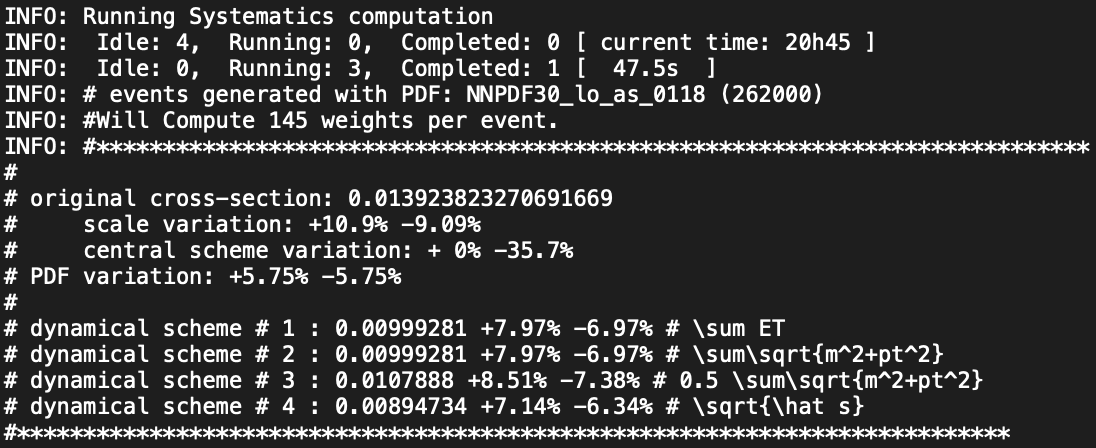
If everything goes well, we should obtain a cross section of 0.0138 pb in a few minutes, with information on two types of uncertainties.
- Scale variations: +10.8% -9.02%
- PDF variations: +5.73% -5.73%
Assignment
Leading-order rate dependence on the neutrino mass
Leading-order rate dependence on the neutrino mass
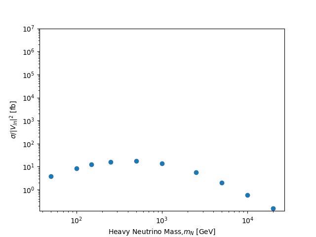
Let’s now repeat the exercise above, but for heavy neutrino masses varying from 50 GeV to 20,000 GeV. After getting enough points, we should generate a plot with the heavy neutrino mass being given on the X axis, and the value of the cross section on the Y axis. Of course, the plot should include error bars as we now have information on them.
In practice, we re-launch the code (by typing launch again), and modify the mass of the heavy neutrino in the param card (line 18). We could perform a scan by setting it to
9900012 scan:[100,5000,20000] # mn1This would perform the calculation three times, the heavy neutrino mass being respectively taken to be 100 GeV, 5,000 GeV and 20,000 GeV. Of course, more than three points should be considered to get a smooth curve.
Summary: uncertainties and production rates at the LHC
In this sixth episode of our citizen science project on Hive, we focused on an LHC signal relevant for a neutrino mass model. We have redone the calculation achieved in episode 5, but this time by including the uncertainties inherent to the perturbative nature of the calculation.
The present episode includes one assignment that should take about an hour to be performed. We want to study the dependence of the neutrino mass signal rate on the neutrino mass, together with the variation of the related uncertainties.
I am looking forward to reading the reports of all interested participants. The #citizenscience tag is waiting for you all (and don’t forget to tag me)! In the next episode, we will re-do that calculation again, but after including subleading corrections to the predictions. We will see that we will get a slightly larger results, but much more precise.
Good luck and have a nice end of the week!


