HiveFest was an amazing experience. I truly enjoyed meeting so many members of our community in person, discussing with them, and obviously chilling with them. In addition, the event also allowed me to shed some light on the STEMsocial project, for which I hope for the best for the current academic year. An app and a meetup may be a good goal, and I will do my best to achieve this!
In the meantime, I now have again (a little bit of) time to start blogging about my research work, and I decided to discuss a scientific publication that my collaborators and I released last June. The article is now under review by the open access journal SciPost (see here), in which even the referee reports and our replies to them are public. Transparency is always the best (I am sure @sciencevienna will agree).
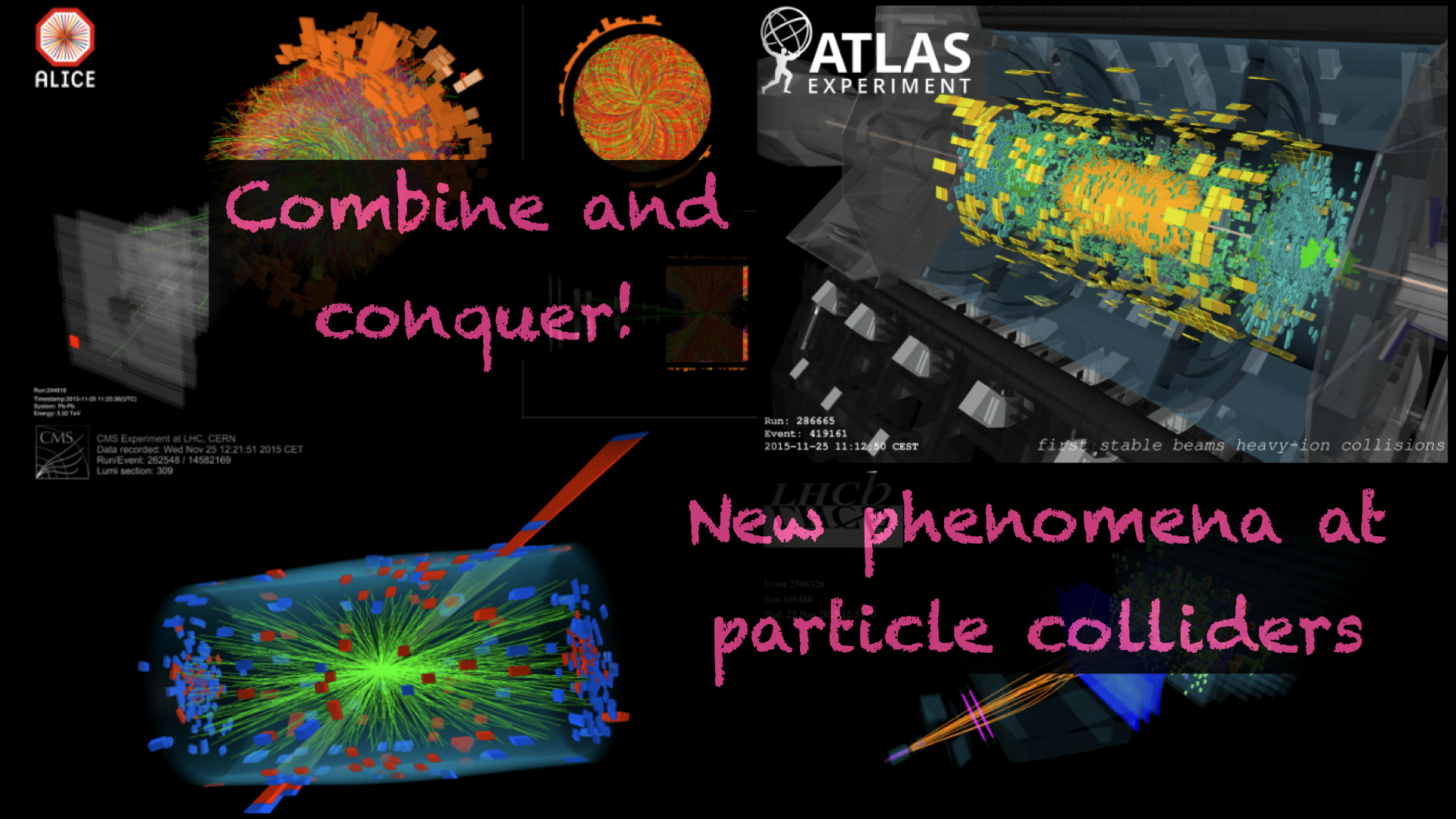
In a previous blog, I discussed how analyses at CERN’s Large Hadron Collider (the LHC) were designed, so that a needle (a signal) could be found in a haystack (the background). Sometimes, it is even more like looking for a specific needle in a needlestack…
[Credits: Original image from CERN]
Despite the complexity of the problem, many searches at the LHC are conducted, and their results are published day after day. This is illustrated in particular on the various wiki pages of the ATLAS and CMS collaborations of the LHC. For instance this page and that page list analyses targeting exotic phenomena.
In all these analyses, the strategy followed to single out a given needle from the haystack is explained, and data and theoretical predictions are compared. Experimental publications indeed show what we expect from simulations, and what we observe from real data. These taken together and compared allow us to extract information either on the exclusion of the existence of something new (the results are compatible with the background), or on a potential discovery (we have an excess or deficit in data).
A big chunk of my work is dedicated to how physicists could reuse experimental results to probe new models. The reason is that there exists a vast world of possible theories that all deserve to be probed, so that experimenters are outnumbered. Because of time and resources, software tools have consequently been designed so that anyone can simulate their own signal of interest, and assess its viability relative to data.
That’s the topic I want to discuss today. In the following, I start with a small summary about how LHC analyses are designed, and then move on with the interpretation of their results. Finally I discuss my last publication and explain what we did to improve the ‘re-interpretation process’ of the published results in the context of new theories, and how this could be made more accurate (and thus better). For those pushed for time, it is OK to directly jump to the last section of the blog (as I somewhat started with a summary).
From 1 petabyte of data per second to a physics analysis
The Large Hadron Collider is a machine in which about 600,000,000 collisions per second occur. It is therefore impossible to store all related information (we are talking about a rate of 1 petabyte per second, or 200,000 DVDs per second). This is however not a big deal, as only a (tiny) subset of all these collisions is relevant to any physics analysis.
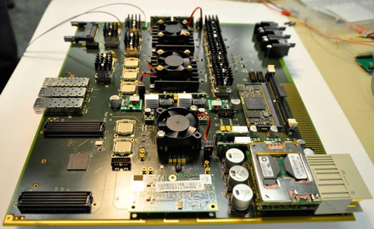
Each detector in the LHC is therefore equipped with a trigger system (see the image below for an illustration) that is capable of quickly deciding whether a given collision is interesting, and thus if it has to be recorded on disk. The decision making process investigates the amount of energy deposited in the detector (the larger the better as we target physics at high energy), and the type of particles that have been produced (boring ones or interesting ones).
[Credits: ATLAS @ CERN ]
Thanks to the trigger system, the rate of recorded collisions is reduced to 200 megabytes per second, which is a quantity manageable by the electronics. We are however at this stage far from any physics analysis, and we need to analyse the corresponding 15,000 terabytes of data per year to study any signal of interest.
This is achieved by starting from the signal we target. Whatever is this signal (it could be associated with pink unicorns, the Standard Model of particle physics, or with any theory beyond the Standard Model), it is associated with signatures in a typical LHC detector. These signatures tell us which kind of subset of recorded collisions (or events) is relevant to us.
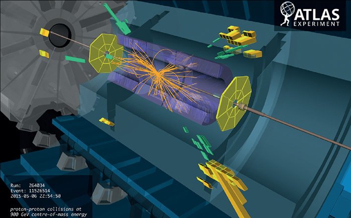
For instance, we may imagine a signal of a theory beyond the Standard Model that leads to two electrons and two muons, or another signal that gives rise to the production of two photons. This defines what we should look for, and therefore the beginning of our selection procedure that will reduce the huge amount of data to something more manageable.
In other words, once we know what we are looking for, we can start selecting events out of what has been recorded, and define a list of requirements. For instance, we may want to select all collisions that have given rise to two energetic photons. We may want these photons to be back to back. We may also require this criterion, or that one, and so on…
We thus come with our list of requirements, and we end up with a small (or at least not too large) number of selected events satisfying them (out of the terabytes of recorded collisions).
[Credits: CERN]
The above procedure leads to observations from data: a number of collisions D satisfy all requirements from our list. It next needs to be compared with predictions, so that we could achieve conclusive statements (in one way or the other). As already written above, the signal could be related either to a process of the Standard Model, or to a process inherent to a theory beyond the Standard Model. This does not matter: we always need to compare data with predictions to conclude.
For this purpose, we perform simulations of our signal, so that we could determine how many signal events are expected to satisfy the list of requirements discussed above.
Next, we have to do the same exercise with the background. In case of a Standard Model signal, the background consists of all other Standard Model reactions, and the corresponding number of events that would satisfy our list of requirements. In case of a new phenomenon, the background is almost the same, with the exception that we consider this time all Standard Model reactions.
Thanks to our simulations, we then know how many background events are expected, how many signal events are expected. In addition, we already know how many data events we have. We can thus run a statistics test, and see whether observations are compatible with the presence of the signal, or not. Both are useful, as this always means that we learn something (in one way or the other).

[Credits: CERN]
Analyses and sub-analyses - a blessing and a curse
Everything that I have written above is true for a given analysis. However, most LHC analyses include several sub-analyses, also known as signal regions.
For instance, let’s take a signal with two photons. We could design a first sub-analysis optimised for a situation where the two photons originate from a new heavy particle. Then, with very minor changes, we could design a second sub-analysis targeting photon pairs that could originate from the decay of a much heavier particle. We need only to adapt a little our list of requirements, which is why the two sub-analyses can be seen as part of the same analysis.
At the end of the day, we may end, after considering many variations of a given situation, with an analysis containing dozens or sometimes hundreds of sub-analyses slightly different from one another. And this is good. Let’s imagine we are looking for a signal of a new particle. We do not know the properties of this particle, in particular its mass and how it decays. Therefore, a large set of sub-analyses must be tried, so that every possibility for the new particle is optimally covered.
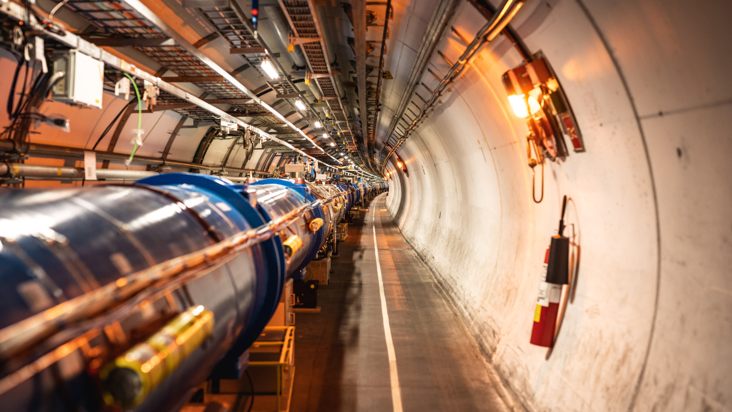
[Credits: CERN]
Having multiple sub-analysis also has another advantage. Let’s assume for the sake of the example that excesses in various sub-analyses would be observed. Taken one by one each individual excess may not be significant, so that data would be statistically compatible with the background hypothesis. However, when taken together, the excesses add up, and we may conclude about the existence of a hint for something new. This is the so-called ‘blessing’ of the title of this section of the post.
On the other hand, the combination of various sub-analyses cannot be done too hastily. There exist correlations, in particular relative to the background and the associated uncertainties, which must carefully be taken into account in statistics tests. This allows us to avoid being overly aggressive (in one way or the other) with our conclusions.
While this combination story is a beautiful one, it comes with a problem (the ‘curse’ of the title of the post): whereas all results published within experimental studies include correlations (as the information is internally known), anyone outside the LHC collaborations cannot handle them properly for the simple reason that related information is generally not public.
As a consequence, anyone outside a collaboration must be conservative, and should only rely on a single sub-analysis in any statistics tests. The subsequent results could therefore be quite off from what could be obtained through sub-analysis combinations.
A paradigm shift - correlation information made available
Recently, experimental collaborations have started to release more information. In particular, information on how to combine different sub-analyses of a specific analysis started to appear. Whilst this is by far not always the case, it is now up to us to show that this information is crucial, so that releasing it, which takes time, gets more motivation and could become systematic.
This is the problem that we tried to tackle in the scientific publication discussed in this blog. We updated a software that I co-develop for many years, so that correlation information could be used when testing the sensitivity of the LHC to any given signal (provided correlation information is available of course). It becomes thus possible to probe a signal by relying not only on the best sub-analysis of the analysis considered, but also on all sub-analyses of this analysis all together.
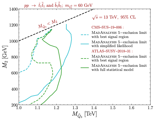
In order to illustrate how this is important, an image is worth 1,000 words. Let’s consider an extension of the Standard Model that includes a few light new particles that decay into each other. To simplify the picture, let’s imagine in addition that the masses of these new particles are driven by only two parameters, that I note M2 and MQ3. Small values of these parameters mean light new particles, and large values heavy particles.
The production and decay of the new particles lead to some signals that can be captured by existing analyses at the LHC. We consider two of them: an ATLAS analysis (ATLAS-SUSY-2018-31) and a CMS one (CMS-SUS-19-006). Each of the two analyses includes many different sub-analyses. The goal is to assess the sensitivity of the LHC to the model by means of the two analyses individually. For a given analysis, we will consider first only the best of its sub-analyses, and next the combination of all sub-analyses.
In other words, for each of the two analyses, we will estimate which pairs of values (M2, MQ3) are excluded when using the most optimal of all sub-analyses, and when combining all existing sub-analyses.
The results are shown in the figure below.
[Credits: arXiv:2206.14870]
In this figure, there are two sets of curves: the green ones related to the ATLAS analysis considered, and the teal ones related to the CMS analysis considered. Every configuration on the left of a dashed line is excluded when we consider only the best sub-analysis of an analysis, the green dashed line being related to the ATLAS analysis investigated and the teal dashed line to the CMS one. In contrast, every mass configuration on the left of a solid line is excluded after the combination of all sub-analyses, for a given analysis again.
As can be seen, combination leads to a substantial gain in sensitivity (we can compare the area to the left of a dashed curve to the area to the left of a solid curve of the same colour to assess this). In other words, combining sub-analyses allows us to probe better the model considered, and to assess more accurately to which parameter configuration the LHC is sensitive.
[Credits: Florian Hirzinger (CC BY-SA 3.0) ]
How to conquer a model better:
By combining, combining and combining!
By combining, combining and combining!
After some exciting days at HiveFest in Amsterdam during which I have met many people who I knew only as a nickname, and even more people who I had no clue about who they were before the party, it is time to resume my series of physics blogs. It is a new academic year after all.
Today, I decided to discuss how analyses at CERN’s Large Hadron Collider are conducted, and what are some of the problems that we face, as physicists, when we try to re-interpret the results of any given analysis in the context of another model of physics.
In general, every single analysis targeting new phenomena includes a lot of sub-analyses, so that any considered new phenomenon could be probed under all its possible facets. The most accurate conclusions are then obtained after a combination of all these sub-analyses. However, as external members of the LHC collaborations, we had until very recently no access to how to perform such a combination correctly.
The situation recently changed, and with my collaborators we updated a public software that I develop to allow anyone to perform this combination, and assess how well their favourite model is cornered by data. Our results are available from this publication, and I have tried to summarise the story in this blog. The TL; DR version is: it works and it is possible.
I hope you liked this blog. Before ending it, let me emphasise that anyone should feel free to abuse the comment section in case of questions, comments or remarks. Moreover, topic suggestions for my next blogs are always welcome.

