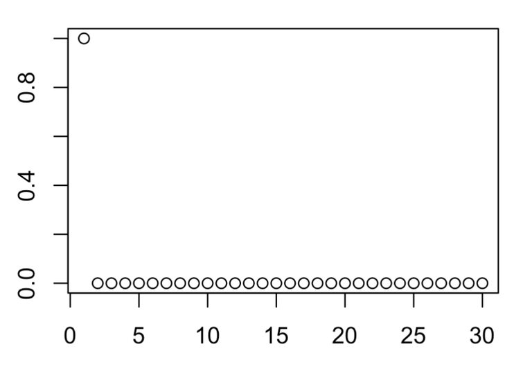
I am just trying to learn the logistic map, so here are some notes and the R code snippets.
Basically what the logistic map does, is a equation that returns the next value based on current value.
The formula is Xn+1 = R * Xn * (1-Xn).
- Xn is the value of X in the nth iteration.
- Xn+1 is the next value of Xn, which we calculate.
- R is the parameter.
This equation has been used in several real life problems to model the situation. One example is population growth.
In its crude form, it looks like this when coding in R.
R=3

x0=0.5
x1=R*x0*(1-x0)
x2=R*x1*(1-x1)
x3=R*x2*(1-x2)
x4=R*x2*(1-x3)
x5=R*x2*(1-x4)
x6=R*x2*(1-x5)
We can try to plot it and iterate over many rounds through a loop.
R=3
a=0.5

points<-c(a)


for (i in 1:30){
  b<-R*a*(1-a)
  a=b
  points[i]<-a
}

plot(points)
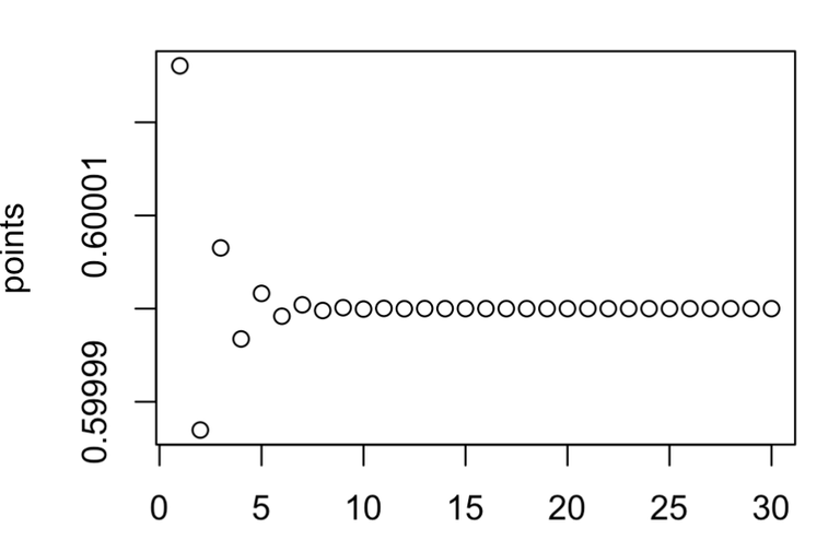
We see a stabilisation with R being 3. This is also call a fixed point when there is a stabilisation to a value.
Let's try with R being 3.4.
R=3.4
a=0.5

points<-c(a)


for (i in 1:30){
  b<-R*a*(1-a)
  a=b
  points[i]<-a
}

plot(points)
Now we see a bistable state, i.e. X value fluctuating up and down.
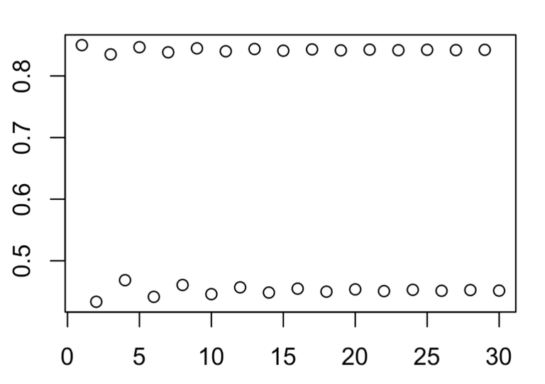
Apparently, at R of approximately 3.5699456, not far from 3.4, something strange starts to happen.
R=3.5699456
a=0.5

points<-c(a)


for (i in 1:30){
  b<-R*a*(1-a)
  a=b
  points[i]<-a
}

plot(points)
The bistable states starts to be changed.
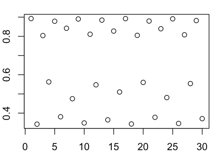
And when R is 3.65, some kind of messy plot emerges.
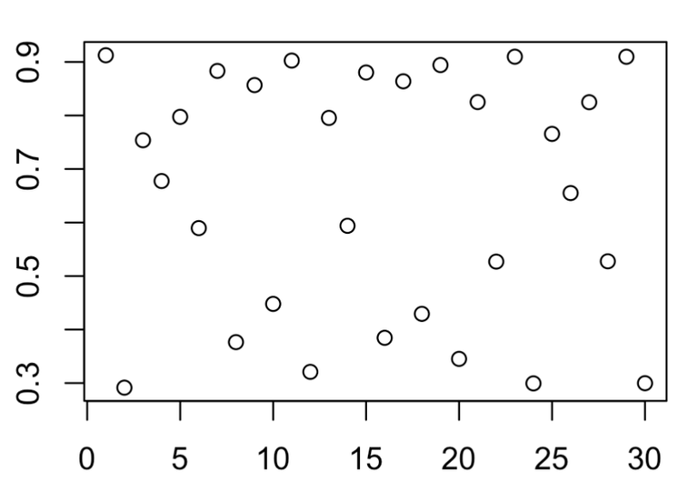
At R at 3.999999999999...
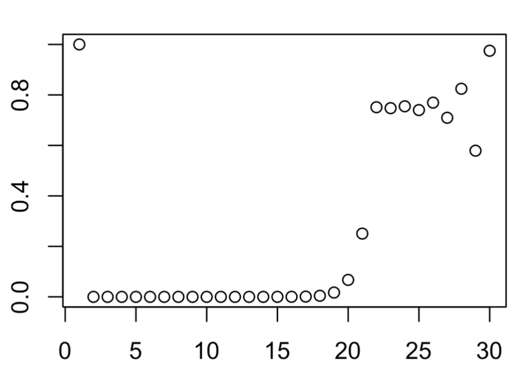
Finally, at R = 4.0. We get back another fixed point.
