After all issues that crossed my way recently, I would have loved to get a calmer moment in the flow of my life. The situation has however not improved, and as a final bonus COVID is now living with us at home. Although I am still COVID-negative (at least for now), the week-end did definitely not allow me to fully rest.
Writing is nevertheless always a good way to disconnect from the on-going burden. I decided today to discuss one of my scientific publications from 2021, that is fully open access for those interested in downloading the actual paper. In this article, two collaborators and I proposed a novel detector simulator that could be used to parametrise the effects of any particle collider detector.
The choice of this weekly topic is not random. Detector simulators consist of a useful subject for the citizen science project in particle physics that is currently on-going on Hive. For those interested, the third episode is scheduled for next week, to give more time to the participants to write their report from last week, and there is still plenty of time to embark with us in this adventure. Please consider having a look to the #citizenscience tag for more information.
Before moving forward, I would like to refer to the two previous blogs that I wrote on particle collider simulations (see here and there). In those blogs, I have explained how we connect a particle physics model to an event, or a specific collision such as those on-ongoing in a particle collider. In this blog, I move on with the natural next step in this process: how to connect a collision to its record in a detector, and how to simulate this on a personal computer.
[Credits: Original image from geralt (Pixabay)]
Particle collision in a nutshell
As detailed in this blog, a particle collision includes several factorisable sub-processes. This means that we can consider them one by one, and thus simulate them on a computer one by one with appropriate numerical tools.
At the inner center of the particle collision lies what we call the hard process, which is where the highest energy is available. The hard process therefore allows for the production of heavy elementary particles that could be either known particles from the Standard Model or hypothetical particles beyond it. For instance, we could consider the production of a top-antitop pair (like in the citizen science exercise of last week) or the production of leptoquarks or supersymmetric particles.
Heavy produced particles then decay, before being subjected to the strongly-interacting environment inherent to a collider such as CERN’s Large Hadron Collider (namely the LHC). This includes parton showering and hadronisation, which can be defined as follows.
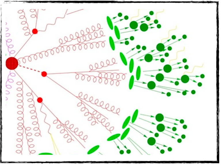
The starting point is that any produced strongly-interacting particle radiates other strongly-interacting particles, that radiate themselves other strongly-interacting particles, that radiate themselves other strongly-interacting particles, etc. At each radiation, a given particle splits in two so that the energy of any individual particle decreases (energy being conserved).
The entire radiation process (in red in the figure below) stops when the energy gets small enough for hadronisation processes to occur. In those hadronisation processes (in green in the figure below), strongly-interacting elementary particles combine and form composite particles made of quarks and antiquarks. These composite particles are generically called hadrons, and known examples include neutrons and protons.
[Credits: A Sherpa artist (image available everywhere in the HEP community)]
In other words, any strongly-interacting particle produced in the hard process or originating from the decay of an unstable particle gives rise to a large number of hadrons. The quantum theory of the strong interaction tells us that all these hadrons are organised in collimated jets of particles more or less flying in the direction of the initial strongly-interacting particle. This is a very useful property that we can use to simplify our vision of the final state of a collision. Instead of considering all the numerous produced hadrons, we apply a clustering algorithm (called a jet algorithm) to cluster all produced hadrons into a small number of higher-level objects called jets.
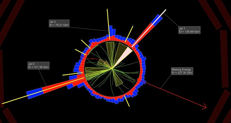
This is illustrated in the figure below that shows a cross section of the CMS detector of the LHC. We can notice a lot of tracks in the detector (in green, in the centre) and a large number of energy deposits (in red and blue, all around the detector). Those come from all the particles produced in the collisions, and in particular from all hadrons. As said above, we can use a jet algorithm to deal with the hadrons and combine them into jets. This is what the yellow cones on the figure do.
The final picture of the collision shown in the figure below gets hence much easier to grasp: there are three jets with a significant amount of energy (see the labels) and some missing transverse energy (also labeled) taken away by Standard Model neutrinos or even dark matter for models of physics beyond the Standard Model. This is a much simpler view than hundreds of tracks and energy deposits left by hundreds of hadrons.
[Credits: CMS @ CERN]
To summarise, whatever is on-going in a real collision, the story always ends with a small number of objects: electrons, muons, photons, missing energy and jets. We can thus classify all produced collisions in terms of the number of electrons, muons, photons and jets that they feature, together with the amount of invisible stuff (i.e. missing energy). Anything else (for instance a Z boson or a Higgs boson) is an unstable particle that always decays into several of these basic objects almost instantaneously.
Detector effects
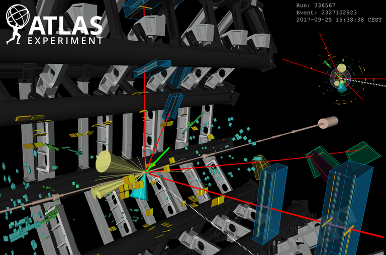
As briefly mentioned above, all objects in which we are interested (electrons, muons, photons, missing energy and jets) manifest as tracks and deposits in a detector. Therefore, the difficulty consists of connecting those tracks and deposits into the initial objects that produced them, so that physicists could have a fair idea of what the final state of any given collision is. In other words, we need to convert a large numbers of tracks and energy deposits in small numbers of high-level objects with well-determined properties.
This is achieved through dedicated reconstruction algorithms, that take as inputs those tracks and energy deposits and return as output high-level objects. This is however not a so straightforward process, because of inefficiencies. For instance, an electron may end up giving rise to few tracks and hits that are not of a good enough quality to be useful.
These inefficiencies could even lead to misleading information implying a bad resolution on the electron’s properties. In the most extreme case, the electron could also end up being totally missed. In this last situation, tracks and hits are present in the detector, but their quality and/or properties do not allow us to associate them with any high-level object.
Finally, there is also the possibility to reconstruct the electron as another object. For instance, electrons faking jets is a possible option. And of course, we can have a situation where for some reason any object of type A is reconstructed as an object of type B.
The above discussion allowed for the introduction of the three big classes of detector effects.
- Reconstruction efficiencies: This corresponds to the probability to actually reconstruct an object from its impact in a detector. This can be a large or small probability, depending on the object properties (its energy, direction, etc.).
- Smearing: The estimation of the properties of a given object is not a perfect science. Inaccuracies are possible, and the actual performance depends on the object properties (again!).
- Identification: There is always a possibility to correctly and incorrectly identify the nature of a reconstructed object. Again, this tagging efficiencies and mistagging rates depend on the object’s properties.
[Credits: CERN]
In order to estimate all relevant probabilities related to detector effects, experimentalists make use of simulations, data and “standard candle processes” that are extremely well known. They fully simulate their gigantic detectors through the GEANT4 package. Such a package allows for the modelling of the detector geometry, that of the interactions with the detector material and it finally includes the simulation of the electronic response of the detector. From there, reconstruction algorithms are put in place to connect tracks and deposits to higher-level objects.
These tasks are however unachievable for anyone who is not part of any big experimental collaboration, mostly due to missing public information allowing to do so. Moreover, achieving it is computationally unfeasible, as it requires minutes of computing time for any single simulated collision. I leave you here with a math exercise, to calculate the resources required for the hundreds of millions of simulated collisions needed by physics analyses… This is really a job that can only be done by experimental groups and their huge amount of available computational resources.
In my work, we introduced a new framework allowing anyone to easily (in terms of computer resources) add detector effects to their simulations.
The SFS framework for detector simulations
In spite of all the potential computer-resource problems related to detector simulators, the probabilities relevant to resolution, reconstruction and identification efficiencies are often released publicly in the form of functions of standard object properties (that are generically called transfer functions). We can thus make use of this to design a computationally more efficient approach than the naive one. The price to pay (there is indeed no free lunch) is that the detector effects are obtained in an approximate manner. However, as long as the approximation is under control, it is fine to use it.
Somewhat, we gain in efficiency for a small loss in precision (which we will keep under control). This is what we achieved in the article that this blog discusses. We coined our framework the SFS framework where SFS stands for ‘simplified fast simulator’.
Our idea was to start from hadron-level simulated collisions, as described above and in the previous blogs on particle collider simulations (see here and there). On each of these hadron-level events, we apply first a jet algorithm. This corresponds to a post-processing of the event final state to determine its content in terms of the high-level object of interest (electrons, muons, photons, missing energy and jets).
In practice, we proposed to make use of the MadAnalysis5 platform as it was capable to handle this reconstruction already automatically. The reason behind this choice is a trivial one: MadAnalysis5 is a package that I co-develop with two friends (one of them being an author of the scientific publication considered today)! By the way, we plan to use this software next week in our citizen science project on Hive.
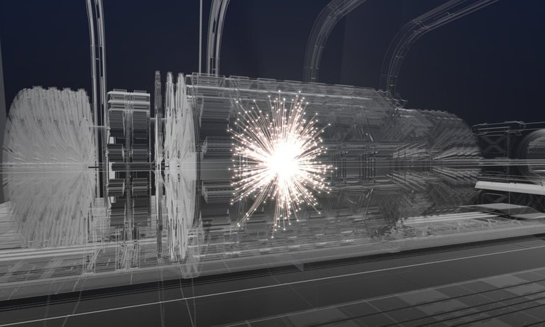
[Credits: CERN]
After running the jet algorithm, we obtain a “perfect collision event” that corresponds to a simulated collision recorded through a perfect detector. This is of course not what we want, and we now need to add all detector effects described above (reconstruction, smearing, identification). To this aim, we extended the MadAnalysis5 framework so that published detector transfer functions can be easily implemented within an intuitive Python-like meta-language.
For instance, the code has now a way in which we could teach it the probability at which an electron with well-defined properties is actually reconstructed as an electron. Moreover, we can instruct it how the electron properties are degraded because of the detector resolution. At the end of the day, it becomes sufficient to take the list of published transfer functions, and implement them directly in MadAnalysis5 so that we could use them to simulate the effects of LHC detectors like ATLAS or CMS.
MadAnalysis5 then automatically generates an associated C++ program that is run. The properties of the different reconstructed objects are smeared, objects can be lost in the process and even change nature. We implemented enough flexibility so that there are very few limitations relative to what we expect from a detector simulator. The “perfect event” is converted into an imperfect one.
Very importantly, we have found that compared with competitor programs, we were up to 50% faster for a much smaller disk-space consumption. On the physics side, results were additionally found in good agreement with the expectation. It is not only important to be efficient; it is also crucial to be physically correct.
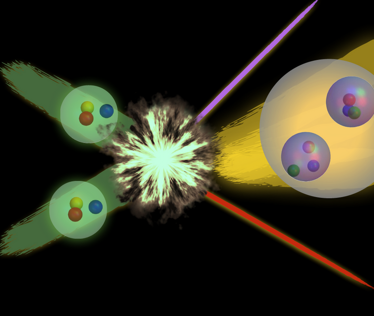
[Credits: OLCF (CC BY 2.0)]
TLDR: a new detector simulator is born!
In this blog, I discussed one of my recent scientific publications. In this article, collaborators and I focused on particle collider simulations, and extended an existing piece of software (that is called MadAnalysis5 and that we develop). The code’s extension concerns a new ability for MadAnalysis5, that is now able to efficiently simulate detector effects.
We implemented methods to deal with all three big classes of detector effects:
- Reconstruction: Any particle that interacts with the detector material leaves into it tracks and energy deposits. Therefore, physicists need to convert tracks and deposits into the objects that generated them. This is always done with some probability, so that there is a way in which the initial object could be lost in the reconstruction process, polluting somewhat our vision of the final state of the collision.
- Smearing: The resolution of the detector effectively yields some smearing on the calculation or on the extraction of any object’s property. Particle physics detectors are not perfect machines, although we built them in order to be as precise as possible. We thus need to provide a way to assess the degradations caused by the usage of imperfect detectors.
- Identification: Finally, the reconstruction of an object from tracks and deposits is one thing. Reconstructing the object correctly is another thing. It may happen that the properties of the object are correctly estimated, but that the nature of the initial object is wrongly recovered. This mis-identification possibility has thus to be included in the simulations, especially as it is more common than what we could naively imagine.
In order to include these effects in particle collider simulations, MadAnalysis5 relies on probabilities obtained from public experimental information. In our approach, that we named the SFS approach, we always give the code a chance to wrongly reconstruct something, lose an object or mismeasure its properties according to published probabilities (that are functions of object’s properties).
We have of course verified that the obtained simulated collisions were in good agreement with the expectation from the LHC detectors, so that the code is ready to be used for real physics project. As a side note, this code is already used by dozens of work and one of the next ones is expected to happen on this chain!
As usual, please do not hesitate to ask me anything (or to provide any feedback) in the comment section of this blog.
I wish all of you a very nice week, and see you next Monday!


